SYMBA Conclusions
This is the concluding and summarizing post to the GSoC SYMBA project. I does not mean that I won’t be posting about it any more, but it’s for the official ending of the GSoC project.
- Introduction
- Data Generation
- Transformer Model
- Training
- Inference
- Evaluation
- Interpretation
- One Caveat: What does the model learn?
- Future Work
- Conclusion
- Personal Conclusions
- Acknowledgements
Introduction
In quantum field theory (QFT) so called “Feynman diagrams” arise naturally in calculation. For example, the scattering-matrix (S-matrix) describes the scattering of particles in QFT. Using Wick’s theorem to get the perturbative expansion (like a Taylor series), each order of the expansion can be represented as a sum of Feynman diagrams. While the expansion can be divergent (as described in one of my earlier posts), they are still incredibly useful and the asymptotic character of the series will only reveal itself directly at orders that probably will never be accessible.
So what can one do with Feynman diagrams? Well, each diagram stands for a specific integral that can be constructed using the Feynman rules for the specific theory you are working with. The diagrams can be interpreted in form of particles that interact, e.g. in the diagram below [from Wikipedia]

an electron \(e^-\) and a positron \(e^+\) come in and annihilate to produce a photon \(\gamma\). This (virtual) photon decays into a quark \(q\) and an anti-quark \(\bar{q}\). The anti-quark emits a gluon \(g\) on its way.
Performing the integral will give you the amplitude \(\mathcal{M}\) of the diagram. Typically \(\mathcal{M}\) will be complex values. This amplitude is complex valued and usually contains lots of Lorentz indices \(\{\alpha, \beta, \gamma, \ldots\}\), \(\gamma\)-matrices \(\gamma^i_{\mu\nu}\) and “basis function” \(u(p, \sigma)\). When I write “squaring the amplitude “ I usually mean more than calculating the norm \(|\mathcal{M}|^2\), but also taking the average over the incoming spins and summing over the final spins. The squaring includes calculating traces over \(\gamma\)-matrices, spin-sums and other tricks, so it is far from trivial. For an introduction and example see Feynman Diagrams for Beginners. With the squared amplitude, one can then calculate measurable quantities. For a scattering process \(2\to 2\) this would be the differential scattering cross section \(\mathrm{d}\sigma(1 + 2 \to 1' + 2' + ... + n')\), see for example here:
\[\frac{\mathrm{d}\sigma_\mathrm{CM}}{\mathrm{d}\Omega} = \frac{1}{64 \pi^2 (E_1 + E_2)^2} \frac{|p_3|}{|p_1|} \bar{|\mathcal{M}|^2}\,,\]where \(E_i\) and \(p_i\) are the energies and momenta of the particles. Similar expressions can be calculated for \(2\to n\) processes. For \(1\to n\) processes, also called decays, the respective quantity is not called scattering cross section, but decay width and usually denoted by \(\Gamma(1\to 1' + 2' + ... + n')\).
These probabilities then help to discover new physics. Say you calculate the cross section \(\sigma\) for some process. It will usually depend on the momenta and energies of the particles. Then you measure the process very often and see that it looks like your predictions except for energies higher than a certain value. What happened? Well, it might be that there is a particle you did not take into consideration in your calculations and that can be produced if energies are higher than the value you found.
Here I am only using two theories: Quantum Electro Dynamics (QED) and Quantum Chromo Dynamics (QCD). While QED describes the electromagnetic interaction between particles, QCD describes the strong force, e.g. holding together neutrons and protons in the nucleus of an atom. This is actually only a secondary effect, QCD describes the strong interaction between quarks and gluon that are present in neutrons and protons. While in our best model, the Standard Model, QED appears in an extended form called Electroweak Theory where the weak interaction, e.g. responsible for the radioactive beta decay, is unified with electromagnetism.
The goal of this project is to teach the squaring of the amplitudes to a neural network. The motivation is three-fold:
- First, to show that it can be done and to explore how it is best done. That it can be done has already been shown in this paper, but I want to explore a different encoding of the expressions called prefix notation.
- Second, to increase the speed of the calculations. Current computer programs for the calculations can take a very long time already for tree level calculations. This of course depends on the optimization of the program and the machine learning model.
- Third, it will be interesting to see how the model performs on expressions where current computer programs will never finish in a reasonable time, e.g. loop calculations or \(2\to n\) calculations with \(n>6\).
Data Generation
In order to generate amplitudes and squared amplitudes MARTY (A Modern ARtificial Teoreteical phYsicist) is used. MARTY is a fantastic program fully written in C++ and can calculate Feynman diagrams up to one-loop in any theory using symbolic computations. The author even wrote the full symbolic computation library (CSL) from scratch in C++. Implementing a new theory in MARTY however is very complicated, thus I am only using QED and QCD. MARTY is built for the symbolic calculation of diagrams, but not for their export. The intended use is to build a C++ library which can then be used numerically. The export of symbolic amplitudes and squared amplitudes can be archived with some tricks, but I had troubles looping over particles. Thus the data generation workflow is the following:
- I wrote a C++ program for the calculation and export of amplitudes and squared amplitudes using MARTY. This program can be called from the command line and takes as input the names of the in- and out-particles as well as the file names where the amplitudes and squared amplitudes should be saved. The program already exports the amplitudes in some form of prefix notation or more precisely in some form of abstract syntax tree. It was easier to do it this way than write a parser in python for them in Python.
- In a separate Python script all combinations of in- and out-particles are calculated and separate processes are spawned calling the C++ script. In order to avoid race conditions with parallelization, each process writes to its own file. This results in a lot of files (28224 for QED 2 to 3 processes), which is probably not good for the SSD and would not be allowed on a cluster, but it’s the best I could do. The squared amplitudes are in a format that can be read by sympy in Python, thus no other steps are done in MARTY/C++.
The generated diagrams are then preprocessed.
Preprocessing
Amplitudes
The amplitudes are rather difficult to handle.
The preprocessing is done in this script.
They contain lots of indices like in the \(\gamma\)-matrices.
E.g. \(\gamma_{\tau, \gamma, \delta}\) reads gamma_{ %\tau_109,%gam_161,%del_161}.
There are also “basis function”, e.g. for the photon \(A_{l, \tau}(p_3)^*\) is represented as
A_{l_3,+%\tau_109}(p_3)^(*).
The following is done in this script to the amplitudes:
- since they are already exported in a nested list structure that represents an abstract syntax tree, the expressions are first converted to a tree and then to a flat list in prefix notation.
- Then the subscripts are fixed. In the expressions above,
%means that a subscript is summed over. We simply remove this information and let the model learn that repeated indices are summed over. Next, the subscripts are converted to a more notation. It does not matter what indices are called if they are summed over, so we convert all greek indices toalpha_iwhere I enumerates them in a given expression. The same is done for roman indices. In QCD capital roman indices are introduces which get their own category. - Finally, the indices need to somehow be encoded.
This is done using the prefix philosopy:
gamma_{alpha_1, alpha_2, alpha_3}is converted togamma alpha_1 alpha_2 alpha_3. This works as long as each symbol likegammaalways has the same number of indices. The basis vectors are endoded similarly:e_{i_1, alpha_1}(p_2)_uis the basis vector for an electron and becomesee i_1 alpha_1 (p_1)_u. Theeeis chosen becauseeis Euler’s number in sympy. For the complex conjugate \(e^*\) a new symbol is introduced for each basis function, e.g.ee^(*).
Squared Amplitudes
For the code see this script for QED.
This step includes simplification of the squared amplitudes and conversion to hybrid prefix notation.
The squared amplitudes are simplified using the factor function in sympy.
Finally, we also combine tokens that frequently appear together to a single token.
This is \(m_i^j\) for \(j=2, 4\) and \(m_i^j s_{kl}\).
It is not stated in the MARTY documentation, but I think \(s_{kl}=-2p_k\cdot p_l\), where
\(p_k\) is the 4-momentum of particle \(k\).
The simplification in sympy can sometimes take a very long time or not terminate at all. I got told that the problem might arise because unlucky random numbers. Thus, there is a timout for the simplification. It turns out that parallelization together with timeouts is not an easy task in Python. For my solution see the blog post on parallel processing in Python with timeout and batches.
Encoding of Expressions
This is the fundamentally new part of my work. In the existing work on SYMBA the strings of the (infix) expressions are encoded using some tensorflow functions I think. Since expressions are actually trees, I think a tree2tree model should perform best. However, this paper on symbolic math with deep learning by people from Facebook, mentions that seq2seq models are good at working with tree structure data. They cite a paper on Grammar as a foreign language and I don’t see the direct connection. Nevertheless, I will leave tree2tree or graph2graph models for future work and focus on seq2seq models here, albeit with prefix notation as also used in the paper mentioned above (the on symbolic math with deep learning), but not in the existing work on SYMBA.
A mathematical expression is fundamentally a tree.
Let’s look a the equation \(a + b*\sin(c)\).
I chose this example because it contains unary and binary operators as we will see.
If we now see all operators like \(+\) as acting on arguments, kind of like you would write
a function in a programming language, then we can for example write
\(a+b\) as add a b.
This way we can see above equation as a tree where the nodes are functions and the
leaves are atomic expressions like numbers or variables.
For above expression we get the tree:
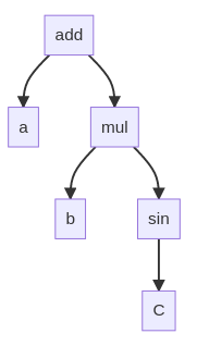
This tree also naturally leads to prefix notation. Perform a depth-first tree traversal and write down everything you encounter. In this example we get:
add a mul b sin c
Now a major problem is this:
The squared amplitudes are large sums.
What happens if we have a sum of many terms?
Say \(a+b+c+d\).
In prefix notation this would be add a add b add c d.
See the problem? So many add tokens.
The computation complexity of transformers scales quadratically with the sequence length.
First: Why do we have to add all those extra add tokens?
The thing is that in order for expressions to be well-defined, every operator needs to have a
fixed number of arguments.
We cannot write add a b c d.
We can easily see the problem in this example:
The two expressions
\(2 \cdot 3 \cdot (a + b + c)\) and
\(2 \cdot 3 \cdot (a + b) \cdot c\)
would be
mul ( 2 3 add ( a b c ) )
mul ( 2 3 add ( a b ) c )
respectively, where I have added parentheses for clarity. If we leave out the parentheses, the two different infix expressions have the same prefix notation. Why not keep parentheses you ask? Because this would give even more tokens, since we would also have them for unary and binary operators.
Hybrid prefix notation:
The way I do it right now is a hybrid between prefix with parentheses and without parentheses.
For add and mul there also exists a new variant, add( and mul( that needs a closing parenthese.
Now, \(a+b\) still stays add a b, but \(a+b+c\) becomes add( a b c ).
Note that for 3 terms in the sum this has the same amount of tokens as add a add b c, but for more
there are no extra tokens added other than the actual terms.
How do I know that this is well-defined?
Basically because I have implemented functions for sympy <-> hybrid prefix and the tests work.
I have tested it on 1000 QCD amplitudes and on some random expressions
like 8*g**4*(2*m**4 - m**2*(s+d)**2).
Right now exp and sin are not working, but they never appear in squared amplitudes.
The sequence length distributions of the amplitudes and the squared amplitudes can be seen below:
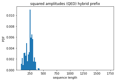
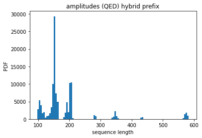
In this project I’ll be capping the sequence length at 350 and throw away all where either the amplitude or the squared amplitude is longer.
Transformer Model
The model I have used is a simple transformer and can be seen in this script. The transformer architecture has conquered the deep learning landscape quickly after the introduction in the famous paper called “Attention Is All You Need”. In the plot below from the same paper you can see the transformer architecture.
![]()
As the name of the paper indicates, transformers are based on the attention mechanism. Explaining attention will take too long for this post, but in short the model learns on which parts to focus its attention. Transformers are sequence2sequence models with an encoder-decoder structure, although other variants definitely exist. Now they not only dominate in language models, but also in computer vision [reference needed].
The code I am using is mostly an adapted version of keras’s english-to-spanish translation tutorial.
I have to admit that I am not satisfied this, but the other parts have simply taken so long that not enough
time was left for a better model.
The transformer has an embedding dimension of 256, a latent dimension of 2048 and 8 heads.
For the maximal sequence length 350 has been chosen.
Usually for language models the embedding dimension is much higher, but I thought since we only have a
rather small number of unique “words” as opposed to the thousands of different words in language translation,
a smaller embedding dimension would maybe make sense.
For tokenization Tensorflow’s TextVectorization function is used, which basically makes a dictionary of all words and enumerates them based on frequency of appearance.
Training
Training is done through next token prediction and categorical cross entropy loss.
Let’s say the amplitude is x and the squared amplitude is y.
Then for each sequence y that is to be predicted, sub-sequences y[0:i], \(i\geq 1\) are constructed
and from (x, y[0:i-1]) the models tries to predict [y[i]].
The sequences y are padded with a [START] token in the beginning and an [END] token in the end.
For optimizer ADAM was used. In the original transformer paper Attention is all you need they have a varying learning rate
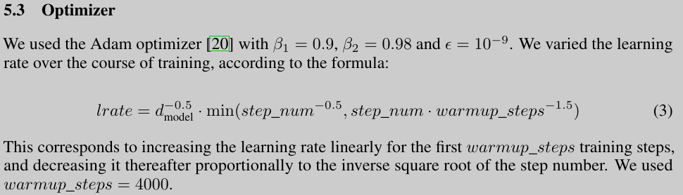
I had also read about super convergence and wanted to try something similar and so now my learning rate looks like this:
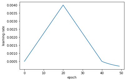
This turned out to work much better than a fixed learning rate.
Inference
Inference is done token by token.
We start with the amplitude and only a [START] token for the squared amplitude.
Then we predict one token after the other, e.g. after the first prediction we would have
[START] add and after the second we would have [START] add 8 and so on.
For each predicted token there is a probability given by the model.
Say for the first token the probabilities are ["8": 80%, "16": 19%, "2": 0.01%, ...].
Then one chooses the “8”, because it has the highest probability.
We stop once the [END] token is predicted or the maximal sequence length is reached.
Evaluation
Viable Evaluation Measures
There are different ways one can measure the accuracy of a natural language model. One possibility is to purely focus on the next token and calculate the next-token-accuracy or the categorical cross-entropy. This is also what the model is trained on.
For machine translation the Bilingual Evaluation Understudy (BLEU)
is usually used.
An extension is METEOR.
Other scores are the ROUGE
or also Perplexity.
Most of those scores are tuned for natural language processing and while our problem
of squaring amplitudes is formulated the same way as natural language tasks, namely as a
seq2seq problem, I think there are differences that justify a different evaluation.
First, we have one correct solution.
There can be different orderings or ways of writing it, but there is only one solution.
Parsing the prediction in sympy and simplifying should get rid of the differences
between two solutions that are written in a different way, e.g. \(a+b\) and \(b+a\)
or \(a(b+c)\) and \(ab + bc\).
Of course here we already have a first test: Can the sequence be parsed into a sympy expression.
Since the predictions are in hybrid prefix format, the first step is to use the
hybrid_prefix_to_sympy
function
that I wrote.
Of course, next token accuaracy is the easiest one to calculate. The next most obvious would be the token score as it is called in the paper. It is defined as the number of correct tokens in the correct position, \(n_\text{correct}\), minus the additionally predicted tokens, \(n_\text{extra}\) divided by the true number of tokens, \(n_\text{true}\):
\[S_\text{token} = \frac{n_\text{correct} - n_\text{extra}}{n_\text{true}}\]Full sequence accuracy: Since we know that there is only one correct solution after simplification, we can simply compare the full sequences. Just count the number of tokens that are at the correct position and divide by the sequence length. Since predicted and true sequence can have different lengths, I propose being conservative and dividing by the longer one. Otherwise it might happen that one of both is much longer than the other and one divides by the shorter one and gets an accuracy of >100%. Let’s call this the “full-sequence-accuray”.
Numerical accuracy: If the sequence can be parsed into a sympy expression, then one can plug numbers into the true and predicted expressions and check the differences in form of (root) mean squared error or mean absolute error. The question is what numbers to plug in. There are two kinds of numbers: Physical constants and the momenta. Physical constants are coupling strengths and masses. They can be either taken as the physical values from measurements or as random numbers. One problem is that the top quark mass is very high and thus wrong predictions regarding the top mass have a much larger impact than say for the electron mass. Nevertheless, plugging in the physical values would give an estimate of what kind of numerical error one would expect in a real application. Plugging in random values would give a better estimate of how well the expressions are reconstructed. For the momenta one has to plug in random numbers. The question is in what range the random numbers should be and what the distribution should be. I have not come up with a reasonable answer yet.
Results
These results are preliminary. I am copying them over from the last blog post.
Here are the last steps of training:
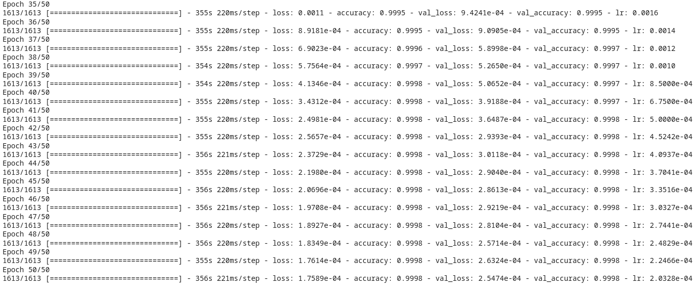
We can see a few interesting points here:
- a next-token accuracy of 99.98% is not bad at all. Assuming all predictions are independent (which is of course not true), this would mean that a sequence of length 350 has a probability of \(0.9998^{350}\approx 93.2\%\) of being fully correct.
- training and validation accuracy are the same, losses not quite,
- in the last 9 steps the validation accuracy didn’t increase, but the validation loss (sparse categorical cross entropy) went down from
3.65e-4to2.55e-4. This is one of the reasons why accuracy is not a good metric. Categorical cross entropy also includes the probabilities the model gives to each token and thus the certainty of the model is included, which the accuracy does not know anything about. Clearly the model continued learning in epochs 41-50, but the accuracy didn’t show this because it was already so high. Probably longer training could help increase performance even more.
I have tested the model on 200 training and 200 test amplitudes.
Inference is standard next-token iterative inference, i.e. one starts with a start token [START] and continues predicting
tokens until the [END] token.
No beam search here.
The token accuracy results are:
- train: 0.9812
- val: 0.9655
Interestingly both are even higher than I had expected from the consideration above.
Interpretation
The transformer model learned to predict the squared amplitudes from amplitudes for QED data with hybrid prefix notation. Thus, my conversions from infix to hybrid prefix notation worked. The token accuracy also is not bad at 96.55%. Still, the accuracy is lower than in the original paper. The differences to the original paper are:
- prefix notation,
- longer sequences, I have used up to 350 and they up to 250. Note that there is a huge difference in predicting 250 or 350 tokens. Say you have 99.98% next-token-accuracy. Then \(0.9998^{250} \approx 0.951\) and \(0.9998^{350} \approx 0.932\),
- hyperparameters: They used 6 layers, 8 heads, 512 embedding dimension and 16384 latent dimension, whereas I used only 2 layers, 256 embedding dimension, 8 heads and 2048 latent dimension. I already have a model with more layers, but training time increases a lot with more layers (I would guess around linearly), so I haven’t finished it yet,
- learning rate schedule.
I’m guessing the longer sequences and the different hyperparameters make a big the difference, so I cannot compare the change in notations yet.
One Caveat: What does the model learn?
I am still not sure about this point. The training data consists of amplitudes and squared amplitudes from processes up to \(2\to 3\). In QED the particles considered are electron, muons, tauons and up/down/strange/charm/bottom/top quarks. The thing is: In QED they only interact through electromagnetism, so there is a symmetry between ALL OF THEM. Let’s say we take the process \(e^- + e^+ \to \gamma + \gamma\), an electron and a positron annihilating and resulting in two photons (one photon is not possible due to conservation of linear momentum and total energy). The amplitude will be the same as for \(\mu + \bar{\mu} \to \gamma + \gamma\) with adjusted massses \(m_e \to m_\mu\) since we are only taking the electromagnetic interactions into account. Since we have so many particles that act in the same way under the electromagnetic interaction, we will get many amplitudes and squared amplitudes that have exactly the same form but with different masses plugged in. Now the question is: Did the model actually learn anything or did it simply remember the structures of the amplitudes and squared amplitudes and what to replace? If so, is this bad or is this what we want? How would this affect completely unseen diagrams?
I want to test this in the future by writing a function to filter out “equivalence classes” in amplitudes and squared amplitudes. Then I can take out a full class of amplitudes from the training data and later test on them.
Future Work
There is still a lot to do. I will continue working on this project even after GSoC.
Compare Notations
The obvous thing to do is to compare infix notation and prefix notation with the exact same model. This will show if it is worth further exploring the prefix notation or not. A full evaluation would include infix, prefix and hybrid prefix data. Of course they will have different sequence lengths. While a comparison between the sequence lengths will be interesting and certainly worth exploring, it will also make the comparison between model performances more complicated. I will have to choose a maximal sequence length for the model, say 350. Then, the models have to be trained on the differently encoded dataset. Best would probably be to have the train/test split done before encoding. Then each model can train on as much training data as it works with (depending on sequence length), but testing should be done on the exact same data (with different encodings of course).
QCD Data
I am working on QCD data and have already calculated amplitudes up to \(3\to 3\) processes, but simplifying them is still a major task. The way my current script does it is:
- load in all the amplitudes and squared amplitudes
- in parallel for batches of amplitude/squared amplitude pairs:
- preprocess the amplitude
- simplify and preprocess the squared amplitude. Timeout if necessary.
- collect the whole batch in one array
- write the array to disk
- continue with next batch
This does not scale to the amount of QCD data, because my 40GB of RAM are not enough. Thus I will have to read in and process in batches.
I plan on repeating the process from the original paper by training on
- QED data alone,
- QCD data alone,
- QED and QCD data.
One of the cool findings of the paper were that the performance on QCD test data improved by adding QED data to the training. I want to reproduce this with prefix notation.
Detailed Comparison Between Sequence Lengths
I want to compare the sequence lengths in infix and hybrid prefix notation for QED and QCD.
More Artificial Amplitudes
When we look at what data natural language translation models are trained on, let’s say the English-German dataset from Anki:
Do you teach? Unterrichtest du?
Do you teach? Lehrst du?
Do you teach? Unterrichten Sie?
Do your best! Gib dein Bestes!
Do your best! Gebt euer Bestes!
Do your best! Geben Sie Ihr Bestes!
Do your best. Gib dein Bestes.
Do your best. Geben Sie Ihr Bestes!
Do your duty. Tu deine Pflicht.
Does it hurt? Tut’s weh?
Does it show? Merkt man es?
Does it work? Klappt das?
Does it work? Funktioniert das?
Does it work? Funktioniert’s?
Does it work? Klappt es?
Dogs are fun. Hunde machen Freude.
Dogs are fun. Hunde machen Spaß.
Don’t ask me. Frag mich nicht.
then we can see that there are lots of short sentences and they often don’t differ very much. We could generate a lot more data by taking some basic building blocks of amplitudes and “squaring” them using MARTY. Let’s call these the “artificial amplitudes” since they are not physical amplitudes. By “squaring” I actually mean taking the squared amplitude of the complex number and calculating the spin sums, which both are not trivial. For example we could square a number or a basis function \(u_s(p)\) and so on. Right now with learning only done on full amplitudes, the model implicitely has to figure out itself what the square of \(u_s(p)\) is. Using the approach with artificial amplitudes would not only generate much more data, but also help the model not overfit on the amplitudes themselves.
Beam Search
For a good introduction to beam search see this blogpost or the “Dive into Deep Learning” book. The idea behind beam search is the following: Instead of choosing the token with the highest probability, choose the top 2 or 3 and “evolve” them separately. It might happen that the first token had a lower probability, but the consecutive tokens have so much higher probabilities, that the total probability (just multiplicate all consecutive probabilities or add their log probabilities) of the predicted sequence is higher than only always going the “greedy” way. Of course, the exact strategies for beam search can vary. A full calculation of all “strains” is usually not computationaly viable, but maybe for the first few steps on can take the top 2 or 3 choices.
Actually I think our use case is a bit different than in a real natural language processing task. Usually in languages there is not one correct solution, but many. Thus, the probabilities can often look like [50%, 20%, 10%, …]. in our case however, the model usually has a pretty high confidence like 99.9%. I propose a different strategy: Every time the model is not sure for a token, say <90%, also take the one with the second highest probability.
Positional Encoding: Symmetries?
Transformers are set2set models, they by default don’t know anything about the order of the elements.
One usually supplies the order through “positional encoding”, which is a whole topic on its own.
The expression we supply have symmetries that are not manifest in the notation.
For example \(a+b\) is represented as sum a b but is the same as sum b a (\(a+b\)).
Now, instead of normal positional encoding, one could implement an encoding where the two tokens a and b
get the exact same encoding in the sequence above.
This way the symmetries could be supplied directly through the positional encoding.
A possible draw-back of this method could be performance. I’m not sure there is a way of implementing this encoding without parsing the expression. I know there is the possibility of learning the positional encoding, so it might also be possible to do pre-training where the positional encoder learns the encoding I describe by forcing it to give the same positional encoding for \(a+b\) and \(b+a\).
Estimation of Uncertainties
I still have to do this, but my idea is the following: For a predicted expression, one can get an extimation of how certain the model is, by multiplying the probabilities for all the predicted tokens. Using test data, I then will compare the certainty with the actual accuracy.
Conclusion
In this project I have shown that a vanilla transformer can learn to predict squared amplitudes in QED if they are encoded in prefix notation. The performance is close to the performance in the paper. I will continue the studies on the topic and explore how well different notations and model architectures influence the quality of predictions.
Personal Conclusions
While I managed to generate data, convert to prefix notation and train models, I didn’t get as far as I planned to. First, writing the programs for data generation took much longer than estimated. This is partly because it took me a few desperate weeks trying to install MARTY until I contacted the developer and he helped me, also fixing bugs in the installer. Then, I had underestimated the complexity of MARTY. I am not a C++ programmer and it took me more than a week to write a command line interface for MARTY in C++ so I can call it from Python and do the rest in Python.
Then, data generation also took very long. Since I wanted the amplitudes in prefix notation and the standard output format cannot be read by Sympy (since it contains indices etc), I had to write functions in C++ to convert the amplitudes to prefix notation (not hybrid prefix!). The squared amplitudes can be read by sympy.
After writing the functions to convert sympy expressions to prefix notation (why is it not possible to get the AST for an expression in sympy???) I realized that prefix notation for long sums and products is counter-productive, see above. Thus I invented and implemented the hybrid prefix notation. While converting expressions from sympy to hybrid prefix notation was rather quick, going back took me a few days. When writing recursive algorithms it’s usually moslty all-or-nothing. It either works or not, but building it step-by-step is often not easy or possible.
Next, reading the squared amplitudes in sympy, simplification and conversion to hybrid prefix, is not as easy as it sounds. It turns out that sympy sometimes gets hick-ups and never finishes the calculation. Allegedly this is because an unlucky draw of random numbers. I implemented functions to stop simplification after a certain timeout time. Connecting this with parallel executions in Python took quite long. Still, on 19 cores the simplification of \(2\to 3\) QED amplitudes takes about a day or longer. Thus I implemented a feature to stop the execution and continue later, because I also needed my PC for things like meetings.
Summarizing I can say that I have learned a lot during this project. I especially enjoyed coming up and implementing recursive algorithms for prefix and hybrid prefix notation. Well, I enjoyed it when it worked xD
Acknowledgements
I want to thank Google for making this Google Summer of Code Project possible. I want to thank Grégoire Uhlrich for MARTY and for the support in installing and using it. Lastly, I want to thank Sergei Gleyzer, Abdulhakim Alnuqaydan and Harrison Prosper for mentoring me.