This is a little update to the SYMBA project.

Data generation

Using MARTY turned out to be much harder than expected. I opted to writing a command line interface in C++ that can be called from the terminal with the in/out particles and file names for export as agruments. The actual loop over the particles is done in Python. One advantage of this approach is the easy parallelizability, since every “process” is saved in its own file. All I have to do is call the program n times in Python.

A potential drawback is the many write processes, since there are very many processes. Possible workarounds would be:

return the amplitudes etc from the C++ file and then process in Python. Would have to look out for race conditions,
cache the amplitudes somehow. Writing to sdtout is complicated I think because of race conditions and also because MARTY writes so much to stdout that I cannot turn off.

Next, the squared amplitudes need to be simplified. Because of the format they are exported, they can easily be imported in SYMPY and simplified there. For making the sequences as short as possible, SYMPY’s factor seems to work best. One problem is that SYMPY sometimes has hiccups and never finishes some amplitudes. I got told this is because of an unfortunate random number, so trying again might help, but right now I simply have a timeout for each simplify.

Representation of equations

The amplitudes contain Lorentz indices and other more comlicated notions, so it’s quite hard to import them in SYMPY. I don’t do more to them than already described in the first post, i.e. exporting in prefix format and some formatting for the indices.

The squared amplitudes however need some work. First, they get converted to prefix notation. This however leaves us with sequence lengths that are way too long. One aid I developed is what I call hybrid prefix notation. Note that we want the notation to be well defined, which I think should be equivalent to the existence of a back transformation to infix notation. Basically we just don’t want two different infix notation equations to have the same prefix notation. This would e.g. happen if we didn’t have a fixed number of arguments for each operator as I showed in the first post. Thus, hybrid prefix notation looks like this:

normal prefix notation without parentheses for all operators except multiplication and addition.
for multiplication and addition, add a closing parenthese, i.e. a+b+c becomes plus( a b c ). Same for multiplication. This way we save one of the parentheses that I had in the first post and also don’t add too many new tokens as in the form plus a plus b c. (Yes, in this example it’s the same amountm of tokens, but for more arguments it’s not.)

However, the squared amplitudes now still have too many tokens. Thus, there are a few tricks we can perform. Basically we add new words to the dictionary in order to save on token length. For lack of a better word I will call this “mass-token-shortening”:

convert all \(m_y^n\) to mny, e.g. \(m_\mu^2\) becomes \(m2mu\),
convert all \(mny * s_{ij}\) to mnysij

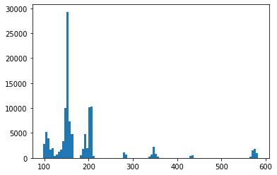
The result is a huge improvement on sequence length. I don’t have a comparison, but for data only on \(3 \to 2\) processes, the sequence length distribution for the squared amplitudes is

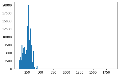
and for the amplitudes it is

Transformer model training

I am using the simplest transformer I could find from a English to Spanish translation tutorial in Tensorflow. Ultimately I want to switch to PyTorch, but this should do as a first model.

The data I am using is \(3\to 2\) QED data, because I had a typo when simplifying the data (wanted \(2 \to 3\)) and it takes around 8h to simplify all the data. I am using sequence lengths in input and output up to 350.

In the original transformer paper Attention is all you need they have a varying learning rate

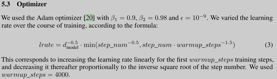
I had also read about super convergence and wanted to try something similar and so now my learning rate looks like this:

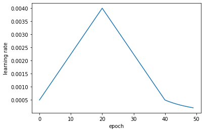
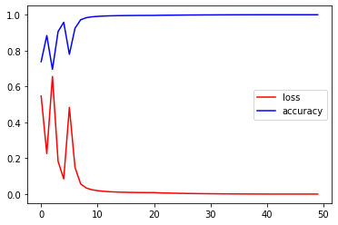
This turned out to work much better than a fixed learning rate. Training of course is done on a next token prediction basis, i.e. the dataset is formated in such a way that the model always sees the whole input and \(n\) of the output tokens. It then has to predict token number \(n+1\). Here are the last steps of training:

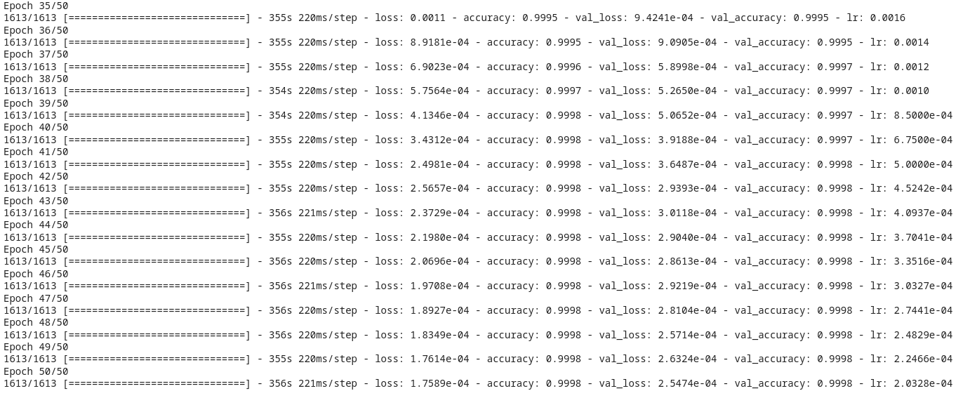
We can see a few interesting points here:

a next-token accuracy of 99.98% is not bad at all. Assuming all predictions are independent (which is of course not true), this would mean that a sequence of length 350 has a probability of \(0.9998^{350}\approx 93.2\%\) of being fully correct.
training and validation accuracy are the same, losses not quite,
in the last 9 steps the validation accuracy didn’t increase, but the validation loss (sparse categorical cross entropy) went down from 3.65e-4 to 2.55e-4. This is one of the reasons why accuracy is not a good metric. Categorical cross entropy also includes the probabilities the model gives to each token and thus the certainty of the model is included, which the accuracy does not know anything about. Clearly the model continued learning in epochs 41-50, but the accuracy didn’t show this because it was already so high. Probably longer training could help increase performance even more.

I have tested the model on 200 training and 200 test amplitudes. Inference is standard next-token iterative inference, i.e. one starts with a start token [START] and continues predicting tokens until the [END] token. No beam search here. As metric I here use what I call “token accuracy”. Basically it’s how many tokens are exactly at the correct position. The results are:

train: 0.9812
val: 0.9655

Interestingly both are even higher than I had expected from the consideration above.

How to quantify certainty of the predictions

In order to later use the model on real data, a measure for the certainty of the model would be good. There are a few ideas that come to mind:

Multiplication of token probabilities: Each token that is predicted comes with a probability by the model. Simply multiplying the probabilities (or maybe adding log probs) would give an estimate of how sure the model is. One could even go so far as to reject results with low probabilities and calculate them classically.
This is also how beam search works. With beam search, motivated by the Symbolic Mathematics Facebook paper, one could do beam search and compare the best results one gets. In the paper they found that their model predicted the same solution, just in different, but equivalent “spellings”. If the model predicts equivalent solutions for the top say 2 or 3 solutions, then it’s also a good indicator that the solution might be correct?

ToDo next:

write a parser for hybrid prefix notation to SYMPY. Once this is done I can numerically check the results by plugging in random numbers. This is one of the metrics used in the SYMBA paper,
simplify \(3\to 3\) data and train model,
generate QCD data,
beam serach and certainty measures,
switch to PyTorch for the transformer model.
graphs with comparison between prefix, hybrid-prefix and hybrid-prefix + mass-token-shortening