Introduction to the Feynman Amplitudes SYMBA Project
This is a little introduction to the Feynman Amplitudes SYMBA project I am working on. It is my Google Summer of Code (GSoC) project and part of the SYMBA project.
Overview and Goals of the Project
I want to calculate Feynman diagrams using Machine Learning! Especially the squaring of the Feynman amplitudes can take a very long time, so the idea is to train a neural network to do this!
Think about it like a machine translation problem, but instead of translating from Spanish to English, it would be from amplitude to squared amplitude or maybe even from some representation of the diagram to the squared amplitude. My group has already published a paper on exactly this, so I don’t have to start from zero. Hakim has already built models for QED and QCD that work remarkably well. I am planing to extend his work. First of all I want to encode the mathematical expressions using prefix notation where Hakim used Tensorflow’s Tokenizer. I also plan to play around with different neural network structures.
Feynman Diagrams
If you have not heared about Feynman diagrams, they look like this:

In the diagram above an electron \(e^-\) and a positron \(e^+\) are incoming. They interact and become a photon \(\gamma\) which decays to a quark \(q\), an antiquark \(\bar{q}\) and a gluon \(g\).
They are so prominent because they fulfill two purposes:
- They arise when doing calculations in Quantum Field Theory in an expansion in the coupling constants. Basically they are a way of drawing the different terms instead of writing down the expressions.
- Feynman diagrams give the expressions in the expansion a picture to look at that is much easier interpreted than the equation. Instead of writing down the integral and doing the expansion, one can just think about the possible diagrams and write them down.
The expansion in Feynman diagrams diverges: Theory of Resurgence
There is some criticism that theoretical high energy physics of the last 50 or so years has been too much focused on Feynman diagrams. For one, they are just very tedious to calculate and there might be better ways of calculating scattering amplitudes. On the other hand, by focusing so much on Feynman diagrams, we might be missing some physics that is not contained in them, or more precicely, that are not contained in a perturbative expansion.
Nonperturbative Quantum Field Theory is very difficult and I don’t know much about it, but I know a bit about the theory of resurgence.
- One can quite easily show that an expansion in the coupling constant has to have radius of convergence of zero! The argument by Dyson in 1953 goes like this: A convergent series in an expansion parameter always converges in a circle in the complex plane around the origin. In Dyson’s example of Quantum Electrodynamics the expansion parameter would be the electron charge squared, \(e^2\) and the expansion takes the form \(F(e^2) = a_0 + a_2 e^2 + a_4 e^4 + \ldots\). It does not matter what exactly \(F\) is supposed to encode here. Now, if \(F(e^2)\) converges, it has to converge in a circle around \(e^2 =0\). But \(e^2<0\) would mean, that like charges attract instead of reflect. Just look at Coulomb’s law. Now, in this world it would be energetically favorable to create a huge amount of electrons and positrons and put all electrons in one part of space and all positrons in the other (see the paper for a longer explanation). Such a world will clearly not be stable. Thus, \(F(-e^2)\) is not analytic and \(F(e^2)\) has radius of convergence zero!
- So why does perturbation theory work at all? It turns out, that divergent series quite often (usually? always?) are better than convergent series! Why is that so you ask? Well, a handwavy argument is this: Divergent series usually are “good” only in a wedge of the complex plane (think between two lines from the origin). Thus, if in the other parts of the complex plane something complicated happens, they don’t have to encode this complicated behavior. Now you might ask: How can a divergent series give something meaningful at all? Or to put it in Abel’s words: “The divergent series are the invention of the devil, and it is a shame to base on them any demonstration whatsoever. By using them, one may draw any conclusion he pleases and that is why these series have produced so many fallacies and so many paradoxes.” This is a longer topic and I intend to write more about it in the future. It turns out that divergent series usually have an optimal order of expansion until which they become better and for higher orders they just get worse until they diverge at infinite order. Also, divergent series usually encode some non-perturbative information, which is the topic of the theory of resurgence, see e.g. Gerald Dunne, lectures by Brent Pym, Daniele Dorigoni or Aniceto, Basar and Schiappa.
What I wanted to say with this litte excursion is: Basing all physics on Feynman diagrams does not give the whole story! Neverteless, my project is about the practical calculations of a huge amount of Feynman diagrams.
The data: MARTY
I will be using MARTY to calculate amplitudes and squared amplitudes. MARTY is an impressive project written in C++. It can calculate amplitudes, squared amplitudes, cross-sections and so on up do 1-loop level.
It took me quite long to get MARTY installed and working. The author was very helpful and always quickly responds to emails!
First, I started with QED.
Since I am bad at C++, I wrote a command line interface for calculating and exporting amplitudes and squared amplitudes.
A typical call would be ./QED_IO.x --particles in_electron,in_electron,out_electron,out_electron for the process \(e^- + e^- → e^- + e^-\).
The amplitudes get saved in files that can be specified with --famplitudes and --fsqamplitudes.
Above call produces the following diagram (I could not get the LaTeX part of MARTY to work, so the labels are missing):

The same diagram also exists for a different channel.
There is also a python script that I use for calculating possible processes for 1→2, 2→1, 2→2 etc. It calculates all potential combination of in and out particles and starts the calculation of the (squared) amplitudes in parallel. A friend of mine noted that saving one file per in/out combination is not good for the SSD and probably collecting the amplitudes and in the end saving them into one big file would have been better, but also more work to code.
Representation of the amplitudes
The amplitude for the diagram above looks like this:
-1/2*i*e^2*gamma_{+%\sigma_73,%gam_55,%eta_12}*gamma_{%\sigma_73,%gam_56,%del_50}*e_{i_3,%eta_12}(p_1)_u*e_{k_3,%del_50}(p_2)_u*e_{l_3,%gam_55}(p_3)_u^(*)*e_{i_5,%gam_56}(p_4)_u^(*)/(m_e^2 + -s_13 + 1/2*reg_prop)
and the squared amplitude:
2*e^4*(m_e^4 + -1/2*m_e^2*s_13 + 1/2*s_14*s_23 + -1/2*m_e^2*s_24 + 1/2*s_12*s_34)*(m_e^2 + -s_13 + 1/2*reg_prop)^(-2)
This is already good, but there must be a better way of representing mathematica expressions than strings. There is a cool paper on Deep Learning for Symbolic Mathematics by Lample and Charton at Facebook AI Research. They teach a neural network to do symbolic integration and solving some differential equations and end up being better than Mathematica in some sense.
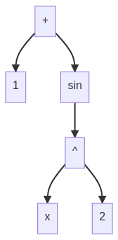
The way they encode mathematical expressions is in prefix notation. Let’s look at the following expression that I just made up for the sake of illustration:
\[1 + \sin(x^2)\]In prefix notation it would be:
+ 1 sin ^ x 2
If you look closely, you can also see that this is equivalent to the following tree:
Later I want to try to use a tree2tree model on this tree directly, but for now it will be a normal seq2seq model. In Deep Learning for Symbolic Mathematics they quickly discuss this. Basically they are saying that seq2seq models work well enough for trees and tree2tree models are slower. However, since the paper probably some new methods for trees (or graphs) have been developed and it might be a good idea to try them.
The way I like to go back from prefix to infix is this:
- Start from the right and go to the left until you reach an operator,
- apply the operator to as many arguments as the operator takes to the right. Note that you need to know the number of arguments for each operator and they have to be fixed,
- what you get is not a fixed block and will be treated as any other element,
- rinse and repeat.
So how would we do it in the example above?
^ x 2→x^2, remaining:+ 1 sin (x^2)(I put “finished objects” in parentheses here)sin (x^2)→(sin(x^2)), remaining:+ 1 (sin(x^2))+ 1 (sin(x^2))→(1 + (sin(x^2)))
Multiple Arguments
MARTY and also e.g. Mathematica or SYMPY like to have multiplications and additions with an arbitrary amount of arguments, i.e. \(a+b+c\) would be + a b c.
The problem with this approach is, that one would then need parentheses for expressions to be well-defined!
For example the two equations
\(2 \cdot 3 \cdot (a + b + c)\) and
\(2 \cdot 3 \cdot (a + b) \cdot c\)
would be
+ (2 3 * (a b c))
+ (2 3 * (a b) c) respectively.
Since in order to save characters I don’t want parentheses, I decided to change multiplication and addition to always take exactly two arguments. Thus \(a \cdot b \cdot c\) will be + a + b c.
My QED_IO.cpp program already outputs the (squared) amplitudes in prefix notation with parentheses. The first amplitude is output in the form
Prod;(;2;Pow;(;e;4;);Sum;(;Pow;(;m_e;4;);Prod;(;-1/2;Pow;(;m_e;2;);s_13;);Prod;(;1/2;s_14;s_23;);Prod;(;-1/2;Pow;(;m_e;2;);s_24;);Prod;(;1/2;s_12;s_34;););Pow;(;Sum;(;Pow;(;m_e;2;);Prod;(;-1;s_13;);Prod;(;1/2;reg_prop;););-2;););
The ; separate the different tokens.
The “postprocessing” of the amplitudes are done in Python.
“Postprocessing” of amplitudes
- convert to parentheses-free prefix notation
- fix subscripts
Parentheses-free prefix notation: Fixing Prod and Sum
In the first step the parentheses are removed and Prod and Sum are transformed to always take two arguments.
For this the input first gets read into a python list, where the ; separate the elements of the lsit.
Then the list gets parsed into a tree using the following algorithm:
- Find rightmost
(, - find corresponding
)by just going to the right until the next), - remove
(and)and put everything between them into its own sub-list, - rinse and repead.
The resulting “tree” is:
['Prod',
  '2',
  ['Pow', 'e', '4'],
  ['Sum',
    ['Pow', 'm_e', '4'],
    ['Prod', '-1/2', ['Pow', 'm_e', '2'], 's_13'],
    ['Prod', '1/2', 's_14', 's_23'],
    ['Prod', '-1/2', ['Pow', 'm_e', '2'], 's_24'],
    ['Prod', '1/2', 's_12', 's_34']
  ],
  ['Pow',
    ['Sum',
    ['Pow', 'm_e', '2'],
    ['Prod', '-1', 's_13'],
    ['Prod', '1/2', 'reg_prop']
    ],
  '-2'
  ]
]
In order to transform the Prod:
- Find a
Prodand count how many elements the sublist, where it is the first element, has, - if only 3 elemets, then pass, but if >3 elements, then:
Prod, second_element, [Prod, third_element, forth_element, ...],- repead for
[Prod, third_element, forth_element]and so on - Do this for all
Prodin all depths of the list.
For Sum it looks the same.
Afterwards we can flatten the list to get this:
['Prod', '2', 'Prod', 'Pow', 'e', '4', 'Prod', 'Sum', 'Pow', 'm_e', '4', 'Sum', 'Prod', '-1/2', 'Prod', 'Pow', 'm_e', '2', 's_13', 'Prod', '1/2', 'Prod', 's_14', 's_23', 'Prod', '-1/2', 'Prod', 'Pow', 'm_e', '2', 's_24', 'Prod', '1/2', 'Prod', 's_12', 's_34', 'Pow', 'Sum', 'Pow', 'm_e', '2', 'Sum', 'Prod', '-1', 's_13', 'Prod', '1/2', 'reg_prop', '-2']
We went from 71 elements to 49 elements by removing the parentheses and adding the needed Prod and Sum to keep it well-defined.
How much saved space should we expect here? Well, it depends on how long the products and sums are.
For Prod ( a b ) → Prod a b we would go from 5 to 3 elements.
For Prod ( a b c ) → Prod a Prod b c we would go from 6 to 5 elements.
For Prod ( a b c d ) → Prod a Prod b Prod c d we would go from 7 to 7 elements and afterwards it gets worse.
However, we are also saving space on all other operations like Sin ( a ) → Sin a.
I have not checked if a hybrid ansatz where parentheses are only used for Prod and Sum would be viable.
Also, it might be enough to only include the closing parenthese and have the opening implicit.
Fixing subscripts
Later I got told that MARTY also has an option csl::option::printIndexIds = false; that surpresses the indices.
I had already created the data (which takes a lot of time) and handled the indices separately, so I’ll stick with
my solution for now:
Let’s look at the following expression for an amplitude:
['Prod',
 '-1/2',
 'Prod',
 'i',
 'Prod',
 'Pow',
 'e',
 '2',
 'Prod',
 'Pow',
 'Sum',
 'Pow',
 'm_e',
 '2',
 'Sum',
 'Prod',
 '-1',
 's_13',
 'Prod',
 '1/2',
 'reg_prop',
 '-1',
 'Prod',
 'gamma_{+%\\sigma_73,%gam_55,%eta_12}',
 'Prod',
 'gamma_{%\\sigma_73,%gam_56,%del_50}',
 'Prod',
 'e_{i_3,%eta_12}(p_1)_u',
 'Prod',
 'e_{k_3,%del_50}(p_2)_u',
 'Prod',
 'e_{l_3,%gam_55}(p_3)_u^(*)',
 'e_{i_5,%gam_56}(p_4)_u^(*)']
Those gamma_{+%\\sigma_73,%gam_55,%eta_12} and e_{i_3,%eta_12}(p_1)_u are what we need to work on.
First, the % signs mean that the index is summed over.
I hope that the model will learn itself that repeated indices are summed over.
Also, if indices are summed over, it does not matter which one is up and which one is down,
so the + can also be removed.
Then we have to think about how to encode the index structure.
I’ll stick with prefix here again, basically for gamma_{+%\\sigma_73,%gam_55,%eta_12} I want the (sub-)tree
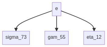
In prefix notation this will look like gamma sigma_73 gam_55 eta_12.
As long as gamma always takes 3 indices this should be fine.
The model should also learn which kind of index comes at which kind of index comes at which position.
For e it will be the same, e_{i_3,%eta_12}(p_1)_u becomes
ee, i_3, eta_12, (p_1)_u, where I have changed e to ee to have it different from Eulers number which also appears in the equation.
For now I have chosen to keep (p_1)_u as one token, but I might have to change it in the future.
The complex conjugate also counts as a seperate token for now:
e_{i_5,%gam_56}(p_4)_u^(*) → ee^(*), i_5, gam_56, (|p|_4)_u.
One last task is left:
There are ugly indices like gam_56 that are all summed over, so their name does not matter.
However, each new index name will be a new word the model has to learn.
Let’s all give them names like i_1, i_2, …, alpha_1, alpha_2, etc for roman and greek indices respectively.
The way we do this is:
- find all unique greek indices in one expression, enumerate them and rename them to
alpha_1, … - same for roman indices →
i_1, …
The final result for above expression is:
['Prod', '-1/2', 'Prod', 'i', 'Prod', 'Pow', 'e', '2', 'Prod', 'Pow', 'Sum', 'Pow', 'm_e', '2', 'Sum', 'Prod', '-1', 's_13', 'Prod', '1/2', 'reg_prop', '-1', 'Prod', 'gamma', 'alpha_3', 'alpha_1', 'alpha_0', 'Prod', 'gamma', 'alpha_3', 'alpha_4', 'alpha_2', 'Prod', 'ee', 'i_1', 'alpha_0', '(|p|_1)_u', 'Prod', 'ee', 'i_3', 'alpha_2', '(|p|_2)_u', 'Prod', 'ee^(*)', 'i_2', 'alpha_1', '(|p|_3)_u', 'ee^(*)', 'i_0', 'alpha_4', '(|p|_4)_u']
Will it be better than using Tensorflow’s Tokenizer? I guess only trying it will show.
Usefulness of this project: How is this better than just building a huge library of pre-calculated diagrams?
It comes down to two points:
- Speed,
- showing that a neural network can learn how to do this kind of analytic math.
The speed is crucial. At tree level, it is not so bad. My parallelized MARTY took around 19h on a laptop for calculating all QED tree level diagrams up to 3 → 3 particles (around 38k, where QED here means electron, muon, tau, up, down, strange, charm, bottom, top, photon and their anti-parts). MARTY can maximally do 1-loop, but already only one process can take a very long time. Squaring the amplitude here takes a huge portion of the time, so if we could make it faster for 1-loop, it could really help. Also, I am not sure if it would even be feasible to pre-calculate all 1-loop diagrams, since they will be so many. For 2-loop or higher I’m guessing computational feasibility and storage might come to their limits, simply because there are so many diagrams and they take so long to calculate. Basically one will be able to choose between only getting the right expression in say 99% of cases, but fast, or correct 100% of the cases and incredibly slow.
Showing that neural networks can do it: It’s clear that they should be able to, but as far as I can tell this is probably the most complicated math ever attempted to solve with neural networks. Included are:
- Integrals,
- complex numbers
- indices
- sums over Lorentz indices and other indices, gamma matrices etc. Group theory in some sense,
- spin sums